TardyGrad: Benchmarking Biologically Plausible Learning Against Backpropagation

Neuromatch Academy — NeuroAI 2026 · Team: M. Miandari (TA), S. Bolotta (TA), D. Picart, V. Chokshi, A. G. Caldeira, L. Valenzuela, B. Bustos, S. Afridi, R. Zhou, J. Reback, J. Tabak

Brains learn remarkably well despite two constraints that backpropagation doesn’t share: rewards arrive late, and neurons can’t send error signals backward through symmetric weights that don’t exist in biology. Project TardyGrad asks whether artificial networks can learn under the same constraints — and which biologically plausible alternatives come closest to matching backpropagation’s performance.

My individual contribution was the Node Perturbation implementation: the full hyperparameter tuning pipeline, the training loop, and the comparative analysis against backprop and Hebbian learning across five seeds.

---

The Problem with Backpropagation

Backpropagation carries three biological implausibilities that prevent it from being a plausible model of how the brain learns:

1. Symmetric weight transport. The forward and backward passes use identical weights — a mechanism that doesn’t exist in biology.
2. Update locking. No layer can update until the full backward pass completes, meaning all layers freeze while the gradient propagates.
3. Downstream error dependence. Every weight update requires knowledge of errors from layers that come after it.

Real biological learning avoids all three. Node Perturbation uses a global scalar reward signal, no backward pass, and no symmetric weights. The question is whether it can match backpropagation’s performance.

---

Three Research Questions

Q1: Can bio-plausible rules match backpropagation on standard MNIST?

Q2: Do they generalize to Spiking Neural Networks?

Q3: How does performance degrade under delayed feedback?

---

Node Perturbation: Learning by Noise

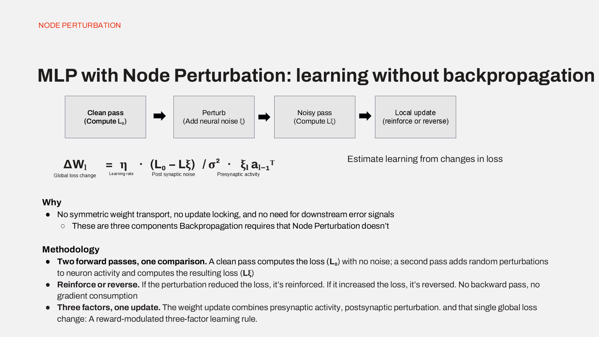
Instead of computing the exact gradient via a backward pass, Node Perturbation estimates it by running two forward passes and comparing the loss.

Clean pass: run the network normally, record loss $L_0$.

Perturbed pass: inject random noise $\xi$ into every neuron’s activation, record noisy loss $L_\xi$.

Update: reinforce the perturbation if it helped ($L_\xi < L_0$), reverse it if it hurt.

$$\Delta W_l = \eta \cdot \frac{L_0 - L_\xi}{\sigma^2} \cdot \xi_l \, a_{l-1}^\top$$

No symmetric weight transport. No update locking. No downstream error signals.

One architectural subtlety worth naming: NP cannot be written as a per-layer custom autograd function, because its update requires a single global number — whether the whole network’s loss improved from this perturbation — and that number doesn’t exist until the full forward pass is compared to the target. The implementation sets .grad directly and lets the optimizer apply it unmodified.

One implementation decision distinguishes this from the course’s reference: noise is injected into the hidden layer’s post-activation firing rate and into the output layer’s pre-softmax logits — not after the softmax, as the reference does. Perturbing pre-softmax keeps the output a valid probability distribution. Perturbing post-softmax doesn’t. An antithetic variant was also implemented, running both $\xi$ and $-\xi$ and averaging the two updates for variance reduction at roughly 2× compute cost per step.

def node_perturbation_step(MLP, X, y, criterion_none, optimizer, generator=None):
    out_clean, out_pert = MLP.perturbed_forward(X, generator=generator)

    with torch.no_grad():
        eps = 1e-12
        loss_clean = criterion_none(torch.log(out_clean.clamp_min(eps)), y)
        loss_pert  = criterion_none(torch.log(out_pert.clamp_min(eps)), y)

        # positive delta_loss = perturbation helped = reinforce it
        delta_loss = loss_clean - loss_pert

        cache = MLP._np_cache
        batch_size = X.shape[0]

        scaled_xi_h    = delta_loss.unsqueeze(1) * cache["xi_h"]   / MLP.noise_std**2
        grad_W1_update = scaled_xi_h.t().mm(cache["X"]) / batch_size

        scaled_xi_out  = delta_loss.unsqueeze(1) * cache["xi_out"] / MLP.noise_std**2
        grad_W2_update = scaled_xi_out.t().mm(cache["h_pert"]) / batch_size

        # BasicOptimizer subtracts grad * lr — negate so it adds the update
        MLP.lin1.weight.grad = -grad_W1_update
        MLP.lin2.weight.grad = -grad_W2_update

    optimizer.step()
    return loss_clean.mean().item()

Hyperparameters were tuned across four stages — sweeping noise_std and lr first on a 3-class subset, then validating on the full 10-class task. The final settings (noise_std=0.15, lr=0.01, 15 epochs) were confirmed across a joint grid. One finding worth noting: on the full 10-class task, the direction of the noise_std effect actually reversed depending on lr — the 3-class heuristics did not transfer, and the optimum had to be discovered independently. Higher lr consistently degraded both accuracy and stability as weights drifted far from initialization, a pattern that held across every condition tested.

---

Results: Full 10-Class MNIST

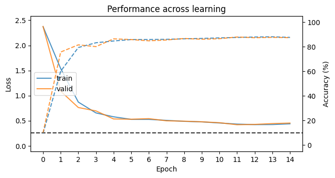
Across 5 seeds: 86.70% ± 0.73% accuracy. All ten digit classes are genuinely learned — no class collapsed.

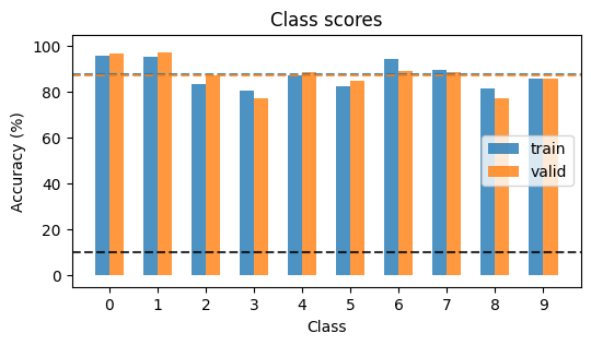
The confusion matrix explains why 3 and 8 are the weakest — and they fail for different reasons.

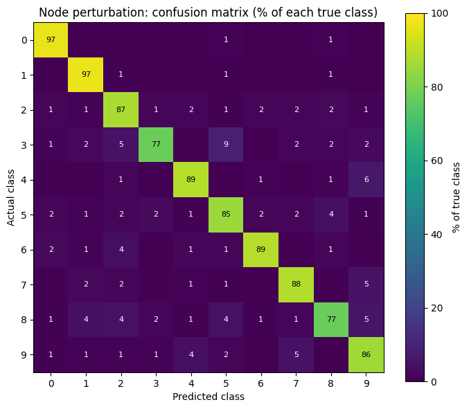
• Digit 3 has one dominant failure mode: 9% of true 3s are predicted as 5 — the largest off-diagonal cell in the entire matrix. A specific, concentrated confusion.
• Digit 8 doesn’t concentrate anywhere — errors spread thinly across almost every other digit. Not confused with one lookalike; just uniformly difficult.
• The strongest asymmetric confusion overall is 4 → 9 (6%) — geometrically sensible, since 4 and 9 share a similar upper-loop stroke in handwriting.

The model’s errors land in intuitively sensible places, which suggests it learned real digit structure rather than a rule-specific artifact.

---

Comparison Against Backprop and Hebbian

Rule	Mean accuracy	Std
Backprop (15 epochs)	92.28%	0.08
Node Perturbation	86.70%	0.73
Hebbian	10.95%	0.00

All pairwise differences were statistically significant (one-way ANOVA F=56,979.7, p≈0; Bonferroni-corrected pairwise t-tests). Node perturbation is meaningfully behind backprop but genuinely functional — it learns all ten classes and generalizes. The ~9× higher run-to-run variance is a direct, expected consequence of estimating gradients from a single random perturbation rather than computing them exactly. Hebbian collapsed to predicting a single class for every input — a qualitatively different failure from “less accurate.”

An honest caveat: this comparison is fair in procedure but not in tuning effort. Node perturbation went through four rounds of hyperparameter sweeps; Hebbian ran at settings tuned for an easier 3-class task; backprop used its original default learning rate, never swept at all. The defensible claim is “node perturbation, tuned, outperformed Hebbian and approached backprop at their existing settings, on this task, across 5 seeds” — not “node perturbation is the better biologically plausible rule in general.” That claim would require giving Hebbian the same tuning effort first.

---

Q1: ANN Results

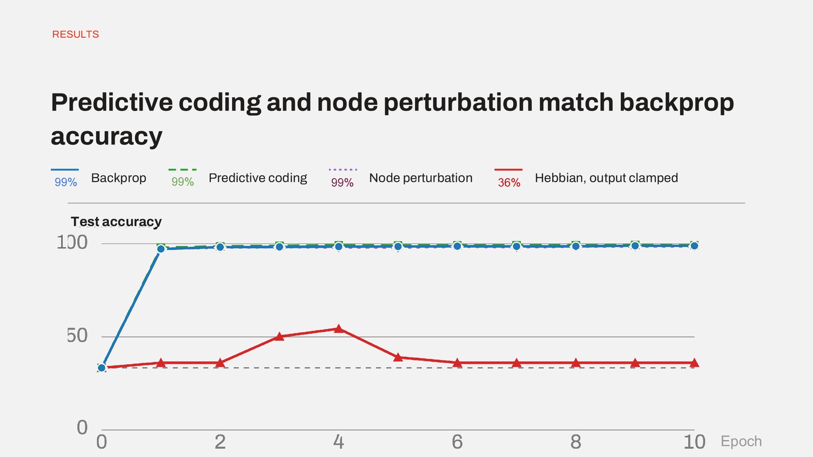
At the team level, both predictive coding and node perturbation matched backpropagation at 99% on MNIST. Hebbian collapsed to 36%. The results confirm that some form of error signal is necessary for learning — but it does not have to be the exact gradient backpropagation computes.

---

Q2: Spiking Neural Networks

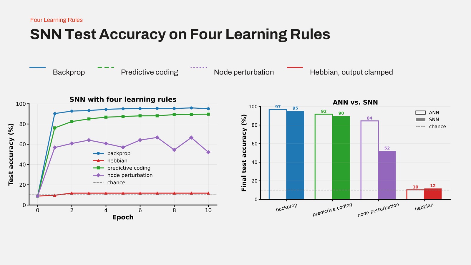
NP’s 32-point drop moving from ANN to SNN is the most striking result in the project. Discrete spiking dynamics make the loss landscape non-smooth — small perturbations produce discontinuous loss changes, making the reward signal too noisy to guide learning reliably. This identifies a meaningful boundary for gradient-free learning: NP works in smooth continuous networks but struggles where discrete dynamics dominate.

---

Q3: Delayed Reward

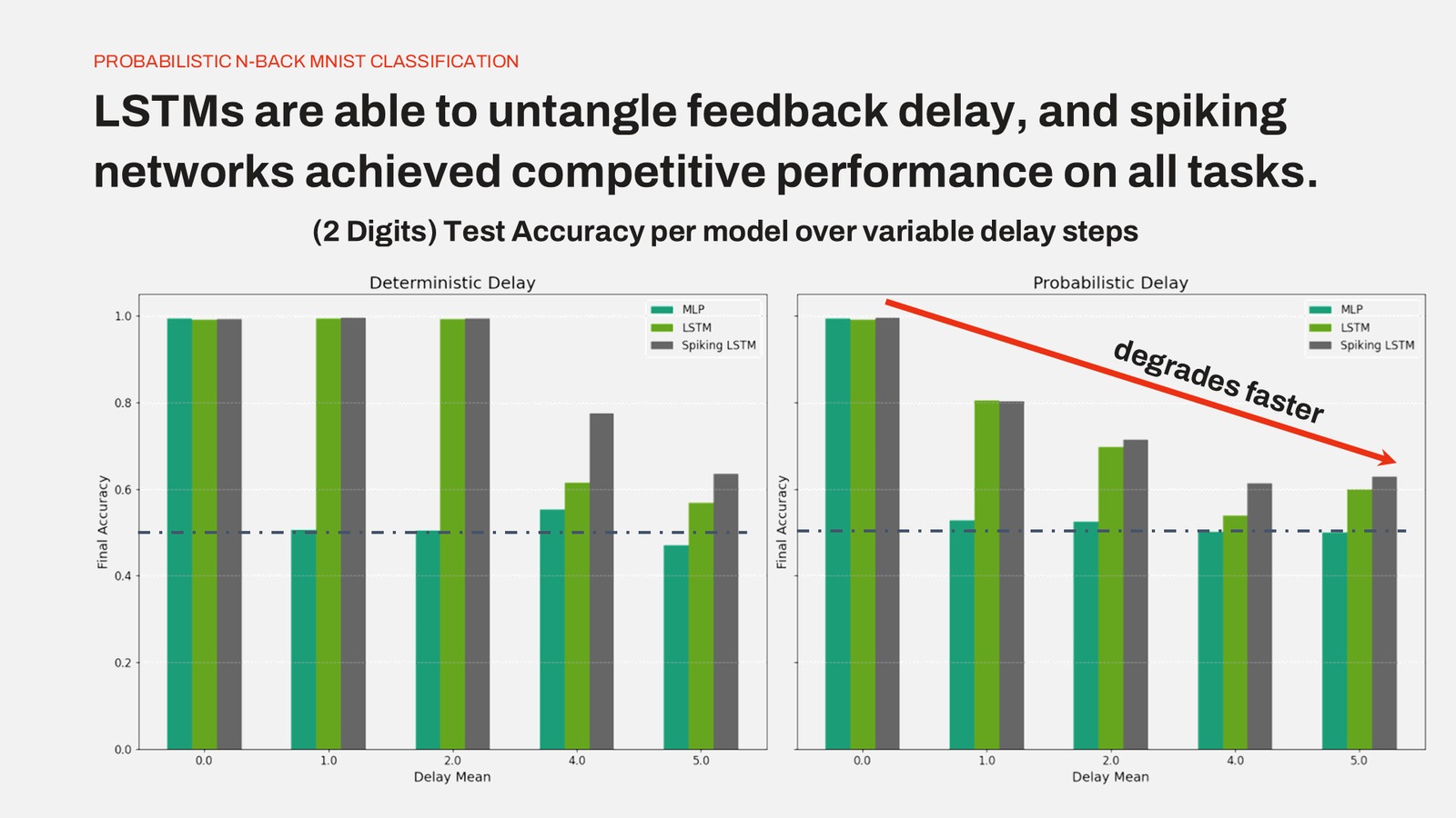
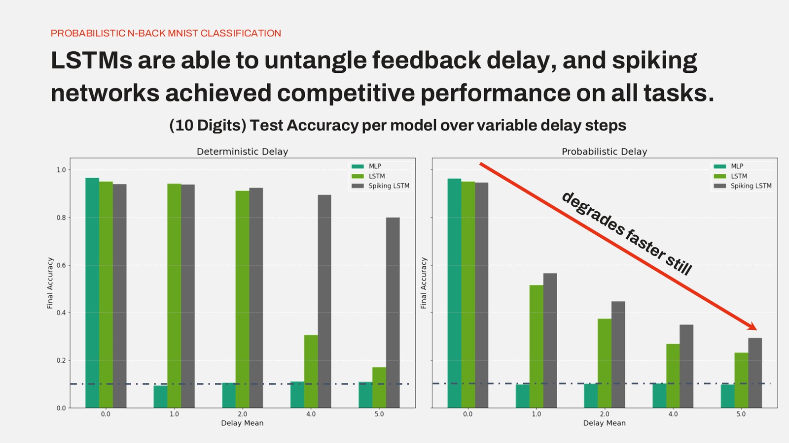
LSTMs handle temporal gaps that destroy feedforward networks. The Spiking LSTM’s advantage grows as the delay lengthens — suggesting that biological temporal dynamics are part of the solution to delayed credit assignment, not just a complication.

---

Conclusions

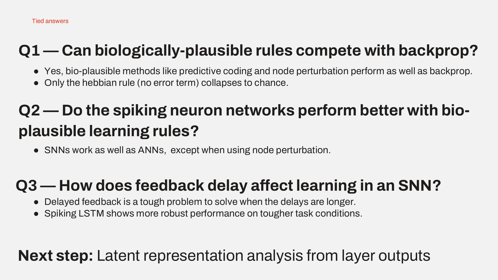
Bio-plausible learning is not one thing. Node perturbation and predictive coding solve the same problem differently, and their failure modes under spiking dynamics and temporal delay are informative about what those differences mean for the brain. The Hebbian rule’s failure shows that a global error signal is necessary — but backpropagation’s exact gradient is not.

---

References

1. Lillicrap, T.P. et al. (2020). Backpropagation and the brain. Nature Reviews Neuroscience, 21, 335–346.
2. Hiratani, N. et al. (2022). Stability and learning in excitatory synapses by a nonlinear mechanism. PLoS Computational Biology.
3. Eshraghian, J.K. et al. (2021). Training spiking neural networks using lessons from deep learning. arXiv:2109.12894.
4. Fernández, J.G., Ahmad, N., & van Gerven, M. (2025). Noise-based reward-modulated learning. arXiv:2503.23972.

Code is maintained in a private repository.