Building a Real-Time School Climate & Equity Analytics Platform
January 15, 2026
PythonSQLYAMLBashJavaScript
Data EngineeringData AnalysisComplianceDevSecOpsPublic HealthOpen DataETL/ELTRAGEquityCloudResearch
Stack: Kafka · Dataproc · Databricks · Snowflake · dbt · FastAPI · LangChain · Chroma · React/TypeScript · Power BI · GCP · Terraform · CI/CD
School climate data (how safe students feel, whether parents trust the school, how engaged teachers are) gets collected once a year, packaged into a report, and handed to administrators who may act on it six months later. By then, the community it describes has already moved. Meanwhile, structural vulnerability data like the CDC’s Social Vulnerability Index updates even less frequently. The result is that the schools most likely to need intervention are the ones whose signals are hardest to read in time to matter.
This platform is my attempt to fix that. It pulls NYC school climate survey microdata in real time, joins it to census-tract-level social vulnerability scores, and makes the combined picture accessible to district leaders through a Power BI dashboard and an AI-assisted Q&A service. The research question underneath all of it: can real-time climate signals predict where structural vulnerability is heading, before the SVI catches up?
1. The Research Questions
The SVI captures structural community conditions: income inequality, housing stability, linguistic isolation. School climate indicators capture real-time social dynamics: safety perceptions, parent engagement, teacher working conditions. These operate on fundamentally different timescales, which creates a genuine research opportunity.
Primary hypothesis: Real-time improvements or declines in school climate are leading indicators of future shifts in community-level social vulnerability. Communities showing sustained climate improvements between 2023 and 2025 are more likely to exhibit reduced vulnerability in the next SVI release. The rationale is grounded in existing research: school climate consistently correlates with family stability, youth mental health, neighborhood safety, and social cohesion — all of which mirror the underlying SVI themes. But the timescale difference is what makes this a predictive relationship rather than a merely correlative one. Climate signals change within weeks or months; structural vulnerability indicators shift over multi-year trends. That lag creates an observation window where climate data can function as a leading indicator, capturing directional movement in community well-being before it surfaces in the SVI.
Secondary hypothesis: Participation rate is itself a vulnerability signal, and one that plays a dual methodological role. Schools and districts with lower student, parent, or teacher participation rates will show systematically lower climate scores and correspondingly higher social vulnerability. Participation is not random; it’s shaped by trust, safety, communication stability, and family engagement, all deeply intertwined with SVI components. This positions participation rate as both a confounder (correlated with both the predictor and the outcome, requiring control) and an independent predictor in its own right. Any model estimating the climate-vulnerability relationship that does not account for differential participation rates will produce biased estimates, because low-participation schools are precisely the ones most likely to underreport poor climate conditions.
Why SVI 2022 Is the Right Dataset
The CDC’s SVI uses specific ACS 5-year windows and is not released annually. SVI 2022, representing ACS estimates from 2018 to 2022, is the current release and will remain so until the next window. This is methodologically appropriate for two reasons. First, SVI measures structural variables (income distribution, housing stability, vehicle access, linguistic isolation, disability rates) that shift over multi-year trends, not single years. SVI 2022 remains analytically valid as a baseline for 2023, 2024, and 2025 observations. Second, the 2018 to 2022 window is uniquely valuable because it captures pre-COVID structural conditions, the acute disruption period, and early recovery, including increased housing instability, displacement patterns, socioeconomic unevenness in recovery, and shifts in employment and healthcare access. All of these directly influence both SVI scores and school climate outcomes. Using SVI 2022 as a multi-year baseline is not a data availability compromise; it is the correct methodological choice for analyzing climate dynamics during the COVID recovery era.
The Four SVI Themes
The CDC scores every census tract across four vulnerability dimensions: Socioeconomic Status (poverty, unemployment, housing cost burden), Household Composition and Disability (elderly, children, single-parent households), Minority Status and Language (racial minority concentration, linguistic isolation), and Housing and Transportation (vehicle access, crowding, broadband access).
NYC’s School Climate Survey captures student, teacher, and parent response rates across roughly 1,800 schools every year, organized into domains: Safety, Relationships, Engagement, and Communication.
The Empirical Plan
Once the platform has three years of climate data alongside SVI 2022 as a baseline, the analysis runs in five steps. First, build a multi-year Gold dataset with weekly aggregates per school covering climate scores, participation rates, and response completeness. Second, join to SVI via a DBN-to-census-tract crosswalk. Third, label districts by trajectory (Improving, Stable, Declining, Volatile) using clustering across the full window. Fourth, test correlations with SVI themes using Pearson and Spearman correlations, participation-weighted regression, mixed-effects models, temporal slope analysis, and multilevel modeling by tract and district. Fifth, attempt to predict future SVI movement. Inputs: SVI 2022 as the structural baseline, climate trajectory slopes as leading predictors, and participation trajectory slopes as meta-predictors accounting for differential reporting bias, with tract-level population weighting throughout. Schools with improving climate and stable or rising participation should align with tracts showing reduced vulnerability in the next SVI release, and the degree to which that alignment holds is the empirical test of the primary hypothesis.
The platform is designed to make all five steps possible, repeatable, and auditable, and to make the results legible to people who will never write a SQL query.
2. The Data Sources
NYC School Climate Survey is an annual NYC DOE survey of students, teachers, and parents. The platform tracks Student, Teacher, and Parent response rates as its primary metrics, along with the underlying survey questions, each tagged with its domain and response scale and stored in the semantic layer so the RAG service can reason over them.
CDC Social Vulnerability Index provides census-tract-level vulnerability scores derived from ACS data. Each tract receives a composite SVI_OVERALL_SCORE (0 to 1) and four theme scores. The platform joins tracts to NYC school districts via census geography, making vulnerability queryable at borough, district, and school granularity.
3. Architecture
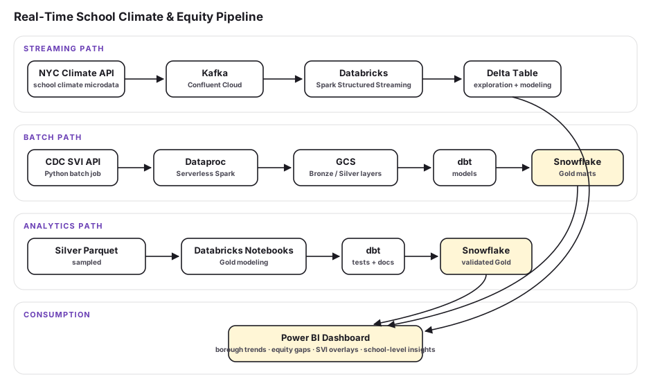
The platform runs three parallel paths that converge at Snowflake Gold.
The streaming path carries NYC climate microdata from the DOE API through Confluent Kafka into Databricks Spark Structured Streaming, landing in GCS Bronze as Parquet.
The batch path carries CDC SVI data from the REST API through Dataproc Serverless PySpark into GCS Bronze and Silver.
Both paths flow into dbt, then Snowflake Gold, where data is modeled, tested, semantically enriched, and ready for consumption.
From Gold, two things are served: a Power BI dashboard for operational visibility, and a FastAPI RAG service for interpretive questions.
4. Streaming Path: Kafka to Databricks to GCS
NYC climate microdata flows into a Confluent Kafka topic using SASL_SSL authentication. Databricks Spark Structured Streaming reads from that topic with micro-batch processing:
raw_stream = (
    spark.readStream
    .format("kafka")
    .option("kafka.bootstrap.servers", KAFKA_BOOTSTRAP)
    .option("kafka.sasl.mechanism", "PLAIN")
    .option("kafka.security.protocol", "SASL_SSL")
    .option(
        "kafka.sasl.jaas.config",
        f'org.apache.kafka.common.security.plain.PlainLoginModule required '
        f'username="{KAFKA_KEY}" password="{KAFKA_SECRET}";'
    )
    .option("subscribe", TOPIC)
    .option("startingOffsets", "earliest")
    .load()
)
Each micro-batch applies deduplication, timestamp normalization, schema enforcement, and watermarking before writing to GCS Bronze. One detail worth naming: the streaming query is explicitly named (queryName("bronze_stream")). An unnamed streaming query caused a null pointer exception in Dataproc’s metrics serializer, a bug that cost more debugging time than the fix deserved.
5. Batch Path: CDC SVI to Dataproc to GCS
The SVI pipeline hits the CDC REST API, validates the response, and writes raw data to GCS Bronze. A Dataproc Serverless PySpark job handles the Bronze to Silver transformation: type casting, deduplication on TRACT_FIPS, and output partitioned by state.
from pyspark.sql import SparkSession
from pyspark.sql.functions import col, to_date, trim

spark = SparkSession.builder.appName("svi_silver").getOrCreate()
df = spark.read.parquet(f"gs://{BUCKET}/bronze/svi/")

silver = (
    df.dropDuplicates(["TRACT_FIPS"])
      .withColumn("COUNTY_FIPS", trim(col("COUNTY")))
      .withColumn("LOAD_DATE", to_date(col("LOAD_TS").cast("string")))
      .filter(col("SVI_OVERALL_SCORE").isNotNull())
)

silver.write.mode("overwrite").parquet(f"gs://{BUCKET}/silver/svi/")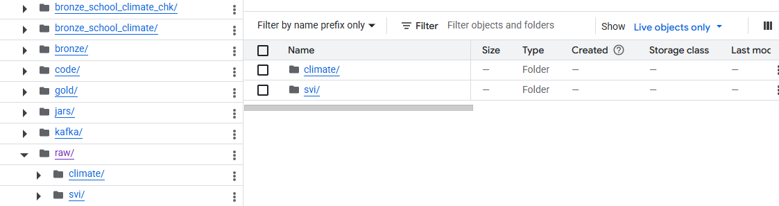
The medallion structure is visible in GCS: raw ingestion folders, Bronze partitioned by source, Silver cleaned and typed, Gold loaded from dbt. Each layer is independently readable for debugging without touching downstream tables.
6. Snowflake and dbt: The Gold Layer
dbt handles all transformations into Gold: schema alignment between the climate and SVI datasets, referential integrity, automated data tests, and versioned models.
# dbt/dbt_project.yml (excerpt)
models:
  school_climate:
    svi:
      bronze:
        +schema: "BRONZE"
        +materialized: view
      silver:
        +schema: "SILVER"
        +materialized: table
      gold:
        +schema: "GOLD"
        +materialized: table
The Gold materializations that matter most for this platform are SCHOOL_CLIMATE_SNAPSHOT (district-level response rate aggregates, the Power BI source), DIM_CLIMATE_QUESTION, DIM_CLIMATE_METRIC_DEFINITION, DIM_SVI_DEFINITION, and GOLD_CLIMATE_VULNERABILITY. Every model has dbt tests for nullability, uniqueness, and referential integrity. The CI pipeline runs dbt compile and dbt parse on every pull request against a dummy Snowflake profile, validating the full DAG without touching the warehouse.
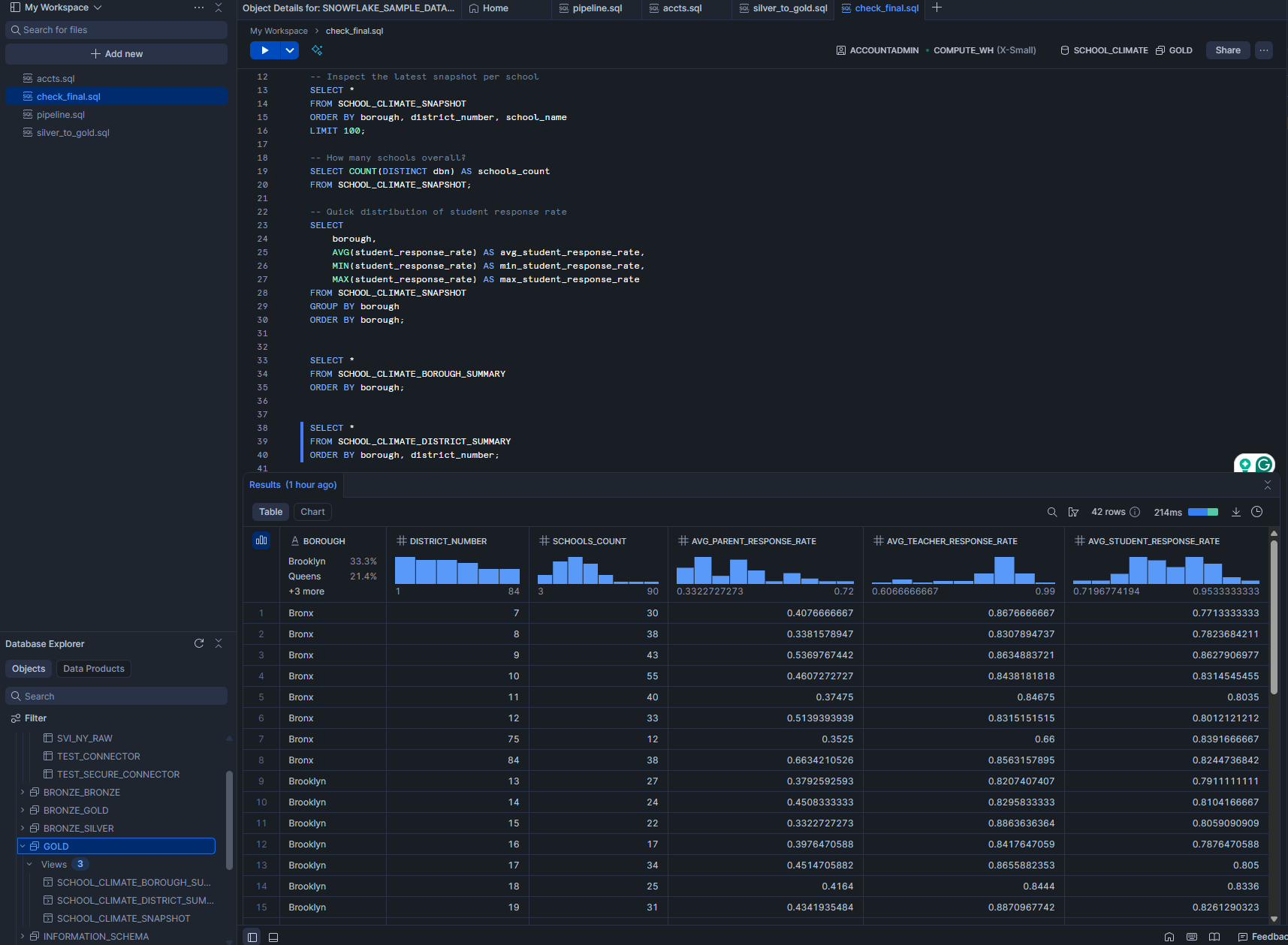
The Snowflake workspace above shows the Gold layer working end-to-end: SCHOOL_CLIMATE_DISTRICT_SUMMARY returning average response rates by borough and district. The database structure on the left (Bronze, Silver, Gold schemas) reflects the medallion architecture in production.
7. The Semantic Layer
The most consequential architectural decision in this project was building a semantic layer alongside the numeric Gold tables. Three dbt-seeded dimension tables describe what the data means, not just what the numbers are.
DIM_CLIMATE_QUESTION stores every active survey question with its plain-language text, survey group, domain, and response scale. DIM_CLIMATE_METRIC_DEFINITION stores metric labels, formulas, and definitions in plain English. DIM_SVI_DEFINITION stores the meaning of each SVI theme and metric, including the bucket logic that categorizes tracts as LOW, MEDIUM, or HIGH vulnerability.
This layer is what makes the RAG service possible. Without it, the AI has numeric values but no language to reason over them. With it, the AI can explain what a metric means, why it matters for a specific community, and how to interpret the number in the context of a district’s SVI profile.
8. Power BI Dashboard
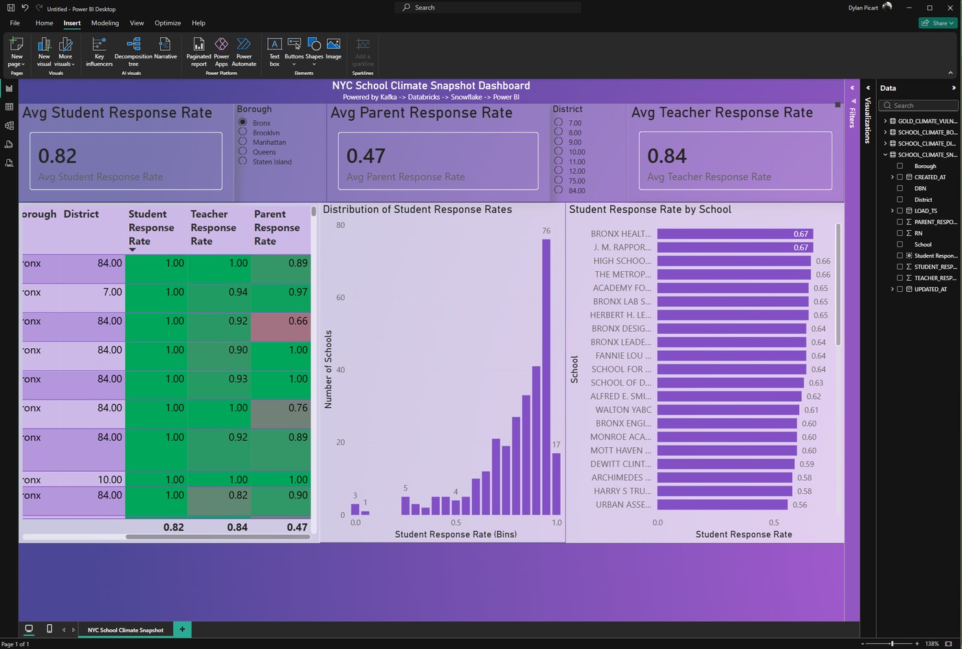
The dashboard answers the operational question: what is happening and where. The RAG service handles the interpretive question: what does it mean, and why.
9. RAG Service: Asking Equity Questions in Plain English
The RAG layer is what separates this platform from a traditional ELT pipeline. A district leader can type “What are the top risk indicators for District 29 schools with high SVI?” and receive a structured, grounded answer that traces back to validated Gold data and cites its sources. No SQL required.
FastAPI → LangChain Retriever → Chroma Vector DB (5K+ docs)
       → Snowflake Gold (live metrics)
       → GPT-4.1-mini
       → Structured response (narrative + bullets + citations)
The Chroma index is built from the four semantic sources: climate questions, metric definitions, SVI definitions, and per-tract vulnerability summaries. Each document is tagged with its source_type so the retriever can distinguish between a definition, a tract score, and a survey question when constructing the prompt.
def format_docs_for_prompt(docs: List[Document]) -> str:
    for d in docs:
        source_type = d.metadata.get("source_type", "unknown")
        prefix_map = {
            "climate_question": "[CLIMATE_QUESTION]",
            "climate_metric":   "[CLIMATE_METRIC]",
            "svi_definition":   "[SVI_DEFINITION]",
            "svi_tract":        "[SVI_TRACT]",
        }
        prefix = prefix_map.get(source_type, "[CONTEXT]")
The Four Query Modes
The API accepts a mode parameter that selects the appropriate prompt template for each type of question.
district_risk_overview connects SVI vulnerability themes to climate metrics for a specific district, returning a plain-language summary and 3 to 5 structured bullets. explain_metric defines a metric, explains its formula, and connects it to SVI patterns. explain_question deep-dives on a specific survey question, drawing from DIM_CLIMATE_QUESTION and DIM_SVI_DEFINITION. compare_districts surfaces similarities and differences between two districts, including caveats about response bias or missing data.
Every response includes citations pointing back to source documents in Chroma and to the Snowflake Gold table that provided the metric, so an AI-generated insight is always traceable.
# POST /api/rag/query
{
  "question": "What are the top risk indicators for District 29?",
  "district_id": 29,
  "year": 2024,
  "mode": "district_risk_overview"
}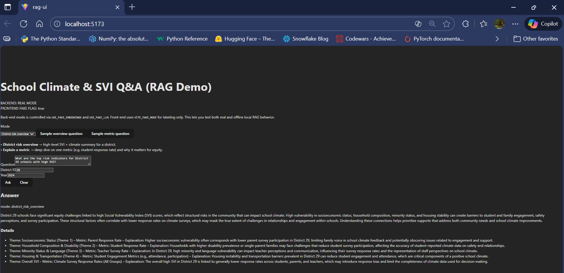
The screenshot above shows the RAG service answering a real query about District 29. The answer connects SVI vulnerability themes (socioeconomic status, household composition, minority status, housing and transportation) to specific climate metrics, explains why each theme may reduce survey participation, and surfaces the equity implications. The mode: district_risk_overview field in the form controls which prompt template runs.
The service ships with a FakeChatLLM for development and CI, returning realistic-looking structured responses without any API calls or cost. Switching to production is two environment variables:
USE_FAKE_EMBEDDINGS=false
USE_FAKE_LLM=false
10. Engineering Challenges
These are the problems that don’t appear in tutorials.
Dataproc CPU quota started at zero. GCP trial projects have no Dataproc CPU allocation by default, so no job can actually start. The fix is straightforward once you know it exists: enable billing, request quota increases for CPUS_ALL_REGIONS and DISKS_TOTAL_GB. Nothing in the error message tells you that’s what’s happening.
Spark couldn’t find the Kafka connector. The error Failed to find data source: kafka appears with no version context. The fix is adding spark-sql-kafka-0-10_2.12 with a version that exactly matches the Spark runtime. A version mismatch is completely silent until execution time.
Kafka JAAS authentication. Confluent’s SASL_SSL configuration for Spark requires an explicit JAAS config string passed as a .option() call. Specifying bootstrap server and security protocol alone isn’t enough. Finding the exact required format took longer than fixing it.
A streaming query name is not optional. Unnamed streaming queries cause a null pointer exception in Dataproc’s internal metrics serializer. Adding .queryName("bronze_stream") to every streaming write resolves it. The ratio of debugging time to fix complexity here was embarrassing.
Databricks couldn’t read from GCS. Cross-cloud restrictions, disabled DBFS, and missing Hadoop connector configs blocked direct reads from GCS in Databricks Serverless. The solution was to export a representative Silver sample, load it manually into Databricks as a Delta table, and treat Databricks as an exploration sandbox rather than a production compute layer. That decision is reflected in the architecture.
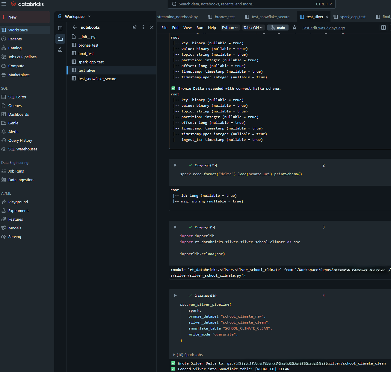
The Databricks notebook above shows the Silver pipeline passing: Bronze Delta reseeded with the correct Kafka schema, the Silver module reloaded cleanly, and successful writes to both GCS Silver and Snowflake. Getting to that green checkmark involved the Kafka connector issue, the cross-cloud restrictions, and schema mismatches between the streaming Bronze and what the Silver transformation expected.
Cloud Shell drops environment variables on idle. Every new session required re-exporting credentials. Wrapping credential exports in a shell script (with the actual secrets in Secret Manager, not the script) solved the session problem.
The GCS networking required a full VPC reset. Dataproc couldn’t write to GCS despite apparently correct IAM configuration. The logs showed Unable to resolve storage.googleapis.com and Connection reset by peer. The root cause was a corrupted default VPC from earlier networking experiments. Deleting and recreating it resolved everything immediately:
gcloud compute networks delete default
gcloud compute networks create default --subnet-mode=auto
The lesson here: networking failures in GCP tend to surface as IAM errors. When permissions look right but nothing works, check the VPC first.
11. CI/CD and DevSecOps
The repository separates CI from CD deliberately. CI runs on every push and pull request: pre-commit hooks covering whitespace, YAML formatting, detect-secrets, black, ruff, and flake8; pytest; dbt deps and dbt parse against a dummy Snowflake profile; and terraform fmt -check with terraform validate. No secrets are used anywhere in CI. The entire validation chain runs clean against stub configurations.
CD is a manual workflow_dispatch workflow. Running dbt against live Snowflake or applying Terraform infrastructure changes requires an explicit human trigger, with credentials loaded from GitHub Secrets at runtime. Deployments are auditable and intentional.
Terraform provisions the full infrastructure from scratch: GCS buckets, IAM bindings, Dataproc configurations, networking, Snowflake warehouse and roles, and Databricks secret scopes. Provider versions are pinned. detect-secrets runs on every commit, enforcing zero credentials in version control.
12. What This Demonstrates
The most interesting thing about this project isn’t any individual piece of the stack. It’s that the research question required the architecture, and the architecture made the research question answerable.
The hypothesis that school climate can act as a leading indicator of structural vulnerability required real-time data ingestion, which required Kafka and streaming. Answering that hypothesis for non-technical stakeholders required a semantic layer, which required the dbt dimension tables. The semantic layer made the RAG service possible, which closed the loop: the research question is now answerable by a district leader in plain English without writing a single query.
That chain from research question to human understanding is the pipeline that matters most.